Ming-Yee Iu
Three-dimensional computer games today render scenes based on a simple pinhole camera model. This technique is fast, simple, and can produce extremely beautiful images. Unfortunately, this sort of rendering provides a very limited field of view. As such, players of computer games are limited to seeing objects directly in front of them in the game world. Seeing objects outside of this limited field of view involves turning the game character to face in a different direction. This is totally unlike human experience and limits the immerssiveness of some games. Although people's vision is also limited to a small field of view, they have 180 degree peripheral vision and are able to quickly turn their heads to get a full awareness of objects completely surrounding them. This sort of "situation awareness" hasn't yet been effectively reproduced in computer games. A fisheye view displays objects within a 180 degree field of view and should help eliminate this problem of limited situational awareness.
Traditional rasterizers based on the pinhole camera model can use simple projective mapping to map polygons onto a flat surface. Fisheye rasterizers involve mapping polygons onto a curved surface. Calculations for this mapping are too intensive to allow for real-time rendering, so numerical approximation and/or warping of other views must be used to speed the rendering. An additional complication is that computer game players are used to hardware acceleration of rendering. Software renderers cannot compete with the speed and quality of hardware rasterizers, so the fisheye rasterizer should ideally be able to take advantage of hardware acceleration to augment the rendering.
This project can help augment the computer gaming experience significantly. Many games such as flight simulators use unwieldy techniques such as multiple views, mouse look, or padlock views to provide game players with situational awareness. Fisheye views are an elegant and intuitive solution to this problem.
There are many different approaches to fisheye rasterization, and comparing these different techniques provide numerous educational challenges. These challenges include
Dealing with image quality issues such as calculating the maximum amount of error allowed in the approximations, dealing with polygon mesh "seams," etc.
The rasterizer will be able to render in real-time 3-d scenes typically found in computer games. In particular, it must render four-sided perspective-correct texture-mapped polygons using a Z-buffer in software only. If the rasterizer is able to achieve these objectives, it will be assumed that it could probably be extended to handle other common game graphics conventions like fog, Gouraud shading, MIP mapping, etc.
Much of the work involved with this project isn't in the creation of the rasterizer itself but in calculating the necessary equations and determining good optimization techniques. Different rasterization techniques must be examined and evaluated for suitability in terms of rendering speed, image quality, and effectiveness and providing situational awareness in computer games. In addition, if time permits, the feasibility of using these techniques for environment mapping might also be explored.
To demonstrate the effectiveness of the rasterizer, a simple walk-through of an animated scene will be made that will be rendered in real-time by the rasterizer.
This project will be based on assignment 3 and will follow a similar layout. It will have gr.c, grsh.c, and util.c to hold model management code, Tcl interfacing code, and generic 3-d graphics routines respectively. Although I had originally intended to use X for displaying images, the primitive image bitblit support in X caused me to choose to use OpenGL for blitting purposes (which is sort of ironic because I'm creating a rasterizer that requires OpenGL to function correctly, but whatever). In addition to the standard modules from assignment 3, there will also be a raster.c to handle software rasterization, a gl.c for OpenGL rasterization, and pcx.c for reading .pcx files.
There are many different types of fisheye views and many different techniques for mapping these views to a 2-d device. The choice of views is important because
Most fisheye views are based on mapping a scene onto a 3-d surface and then mapping this 3-d surface to a 2-d screen. The most common 3-d surfaces used in this way are paraboloids and hemispheres.
A paraboloid is useful because a 180 degree view can be generated from a parboloid merely by taking an orthogonal projection of the surface onto a 2-d screen. There is also a reasonable amount of detail in all parts of the image, and the resulting circular image is easy for the user to interpret.
The formula for the surface is
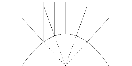
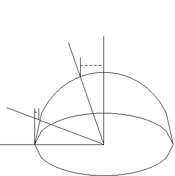
In order to rasterize efficiently, we want to walk across the image in a horizontal or vertical line. As a result, we will end up sweeping across the surface of the paraboloid in a straight line. As we perform the sweep, we should examine the direction we are rasterizing in.
In the above diagram, we have a picture of a paraboloid with dashed lines indicating the line of the paraboloid that is being rasterized. The vertical dashed line is the orthogonal projection vector that is being used to rasterize.
The rasterization direction is in the same plane as the orthogonal projection vector. As such, a vector that is perpendicular to the projection vector and the normal is also perpendicular to the rasterization direction vector.
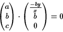
If
![]() is the perpendicular vector then
is the perpendicular vector then
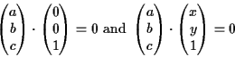
Solving this, we get a perpendicular vector of the form
Since the rasterization direction vector is perpendicular to that, we can derive some information about the direction vector
The perpendicular vector can be of any length, but is definitely not
![]() ,
so let b arbitrarily be 1.
,
so let b arbitrarily be 1.
In addition to this, the rasterization direction vector is symmetric about the surface normal with the orthogonal projection vector. (Assume u is the orthogonal projection vector, v is the normal, and w is the rasterization direction.)
The v cancels out and assume w is a unit vector.
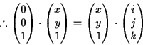
Solving for i, j, and k, we get a rasterization direction vector of

So, if we attempt to rasterize a row of pixels, we would hold y constant and change x. By doing this, the rasterization direction vector will trace a curved pattern. If we rasterize polygons in this way, we will move across the polygon texture map in a curved pattern which is inefficient and difficult to optimize.
Ideally, we want to be able to intersect both the 3-d surface and the polygon to be rasterized with a plane, and have all the rasterization direction vectors at those locations lie on this plane. If this is possible, then we will be able to rasterize the surface using straight lines AND walk across the texture map of the polygon in a straight line. Working on a plane also has the advantage that the rasterization problem then degenerates into a 2-d problem rather than a 2-d problem. One way to do this with a paraboloid is to take planar cuts that cross through the center of the paraboloid (i.e. through points (0, 0, 0) and (0, 0, 0.5) ). Unfortunately, rasterizing a view in this way leads to an extremely distorted image that probably doesn't have any parallel in the real world and is hence difficult for users to understand. This technique will be useful in rasterizing the hemisphere however.
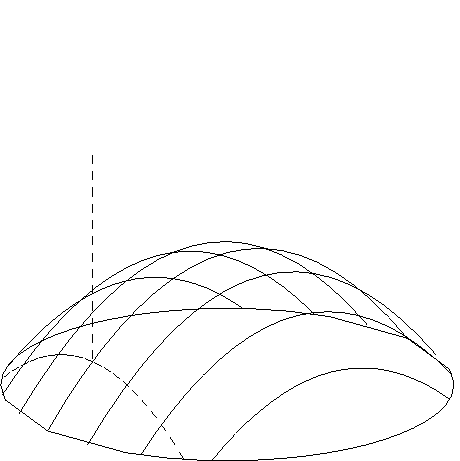
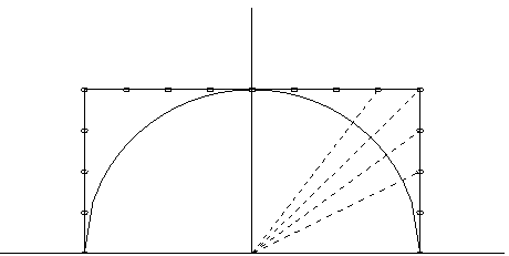
The other common 3-d surface used to generate fisheye views is the hemisphere. Like the paraboloid, a 180 degree view can be generated by taking an orthogonal projection of the surface onto a 2-d screen. Unfortunately, an orthogonal projection mapping leads to poor detail in the resulting image near the edges of the hemisphere. As can be seen in the diagram below, the same "area" of scenery of the hemisphere can map to very small surfaces after a projection mapping.
Instead of taking a direct orthogonal projection, it is more efficient to take planar slices of the hemisphere and rasterizing each of these slices separately. If we take these slices at regular angle intervals, we will then get consistent level of details for each slice along one axis. There will be considerable amounts of redundant information near the edges of the slices, but this extra detail isn't as much of a problem as lack of detail at the edges. By rasterizing each slice separately in this way, we get a rectangular image of what's on the hemisphere.
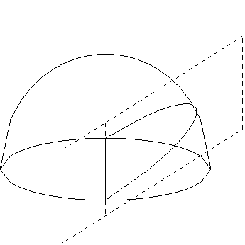
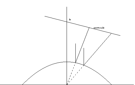
So, we have now reduced the problem to a 2-d problem of projecting a line onto a circle. For this mapping to be effective, there must be a way of efficiently generating accurate polygon Z-values for the Z-buffer. Below is a picture of one of the planar cuts of the hemisphere.
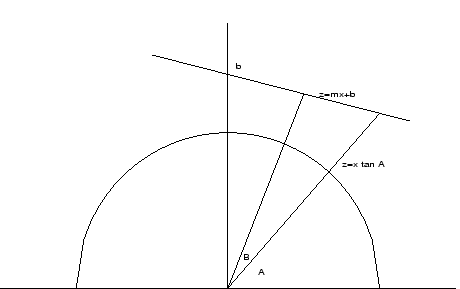
We want to "sample" the polygon at regular angle intervals. We will start with A=0 and increase it by a fixed amount until we reach the end of the polygon. To properly get polygon depth ordering, we should calculate the distance of each polygon from the center of the hemisphere. This results in a messy formula with multiple trigonometric functions. Instead we will use the Z distance as a distance measure. In general, if a point has a greater Z distance, it is further from the center of the hemisphere. The Z values are not a good indicator of distance, however, when Z is close to 0. To avoid this problem, when the angle is below 45 degrees and above 135 degrees, the x value will be used as the distance measure. At these angles, a greater x value is equivalent to being further away from the center of the hemisphere. This switch is necessary because these distance measures must be as accurate as possible because if depth ordering is incorrect, rendering errors will appear in the image which are usually easy for people to spot.
Since the derivation of equations is long, we will only examine the case where Z values are used as a distance measure in the range from 45 degrees to 135 degrees (working with the x values in the other angle ranges results in similar equations and follow a similar derivation).
Let ![]() be the angle of the sweeping rasterization line (this is A in the above diagram).
be the angle of the sweeping rasterization line (this is A in the above diagram).
As ![]() is increased from 45 to 135 degrees, z changes in a very non-linear fashion. As such, calculating z values in this way cannot be optimized easily. Instead, let's look at
is increased from 45 to 135 degrees, z changes in a very non-linear fashion. As such, calculating z values in this way cannot be optimized easily. Instead, let's look at
![]() .
.
If we use 1/z as our distance measure for the Z-buffer, the Z calculation for each pixel will involve one multiply and one add (assuming that we implement ![]() using a look-up table). This isn't too bad. High end processors like the Pentium III have pipelines which can dispatch one multiply per cycle. Still, if we could use only a series of additions on each pixel, the algorithm would be usable on a much larger range of processors. To do this, we can approximate the curve with a piecewise linear function (quadratic functions could also be used, but for simplicity, I'll start with a linear function).
using a look-up table). This isn't too bad. High end processors like the Pentium III have pipelines which can dispatch one multiply per cycle. Still, if we could use only a series of additions on each pixel, the algorithm would be usable on a much larger range of processors. To do this, we can approximate the curve with a piecewise linear function (quadratic functions could also be used, but for simplicity, I'll start with a linear function).
SIDE NOTE: It is interesting to see that 1/z uses a cot (bounded to within -1 and 1 when calculated within the [45, 135] range) while 1/x gives a tan (bounded to within -1 and 1 when calculated within the [0, 45] and [135 180] range). This is convenient since it avoid the numerical problem of having a function grow to infinite.
As mentioned before, it is crucial that the distance values be as accurate as possible, so if we are approximating it, we must get some bounds on the approximation.
So f(x) is the cotangent term of 1/z (we'll ignore the constant term for now).
We want to approximate the curve between ![]() and B. So the error of a linear approximation between those 2 points is
and B. So the error of a linear approximation between those 2 points is
![\begin{align*}f(t)-\left[t\left(\frac{f(B)-f(0)}{B}\right)+f(0)\right]\\
=k\cot...
...rac{t}{B}\cot\theta - \cot\theta - \frac{t}{B}\cot(\theta+B)\right]
\end{align*}](img27.gif)
Let's differentiate by t and set it to zero to find the max and min.
Because t>0, ![]() .
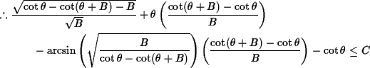
Therefore, we need only consider the positive case. From here, we can substitute back into the original equation, set and error bound on it, and isolate B to find out how big we can make our piecewise linear approximations. Let C be the error bound.
.
Therefore, we need only consider the positive case. From here, we can substitute back into the original equation, set and error bound on it, and isolate B to find out how big we can make our piecewise linear approximations. Let C be the error bound.
This looks really hard to solve, so we type it into Maple, but Maple cannot solve it. Maple also cannot solve rough approximations of this equation. Usually, this would mean that we would be stuck. Fortunately, though, if we graph everything in MatLab, we can see that tan and cot are close to being linear on the ranges that we use them for. In fact, approximating the whole curve with just a single linear equation results in only a maximum of about 10
So with these linear approximations, how many multiplies must we do? Each linear approximation can be calculated with one add per pixel; therefore, multiplies will only be needed when switching between different pieces of the approximation. The number of multiplies is proportional to the number of pieces in the approximation. More pieces will be needed for those lines which are close to the viewer or those with steep slopes (as can be seen by examining the coefficients of the cot that we are attempting to approximate). This is reasonable because the polygons are either close to the viewer (and hence, should be approximated carefully) or are viewed on edge (and hence, are usually very thin and can be drawn quickly).
The equations needed to perform texture mapping can be calculated in a similar way, but its accuracy is less critical because small imperfections in the texture aren't too noticeable. Instead, the common technique of linearly approximating the texture in fixed step sizes can be used.
Although the hemisphere mapping can probably be implemented, it still suffers from some small errors in its distance calculations, and it is somewhat difficult to implement. By combining some of the features of the paraboloid and the hemisphere, it is possible to create a new shape that might be easier to rasterize. The hemisphere is useful because planar cuts of the object can be made, allowing the problem to decompose into a 2-d problem. Unfortunately, the trigonometric functions in the resulting problem is difficult to calculate efficiently. On the other hand, the paraboloid is a shape involving no trigonometric functions, but planar cuts of the shape do not help decompose the problem into 2-d.
Taking the best features of both shapes, we can create a shape that we are able to take planar cuts of (similar to the hemisphere) and where each cut results in a 2-d problem involving mapping polygons onto a parabola. One shape that satisfies these constraints would be a parabola that is swept in a circle. This shape does not have any official name, though it could probably be called a swept-parabola or parabolosphere or hemi-spherabola. The actual shape, of course, is irrelevant. The important thing is how good the shape is at generating fisheye views.
The above figure shows the problem of mapping a polygon onto parabola and then using an orthogonal projection to map the parabola to the screen. The parabola is defined by the equation
The orthogonal projection vector is
![]() .
Depending on which point on the parabola we are performing the projection for, the tangent vector at that point is
.
Depending on which point on the parabola we are performing the projection for, the tangent vector at that point is
![]() .
The rasterization direction vector
.
The rasterization direction vector
![]() is the same angle from the tangent vector as is the orthogonal projection vector.
is the same angle from the tangent vector as is the orthogonal projection vector.

So far, so good. But this still isn't fast enough. Although each individual scan line can be drawn quite quickly, setting up each scanline to be drawn requires a considerable number of calculations. In particular, we need to calculate where the polygon being rasterized intersects each scan line in order to draw the scan line. Under traditional projections, straight lines map onto straight lines, so the intersection across all the scan lines is a straight line, which is quite easy to calculate (you take an edge of the polygon, and map it onto a straight line on the screen, and as you move down scan lines of the screen, you just move to the next point along the straight line as your intersection with the scan line). Unfortunately, things are not so simple under a projection onto a hemisphere-paraboloid. So what exactly do straight lines map onto under this projection?
Firstly, we have to calculate points are mapped. Suppose we have a point (x,y,z) and we want to know what the x-position of that point on the screen is. Recall from before that we used t to represent the x-position on the screen. Well, to calculate the x-position, we first intersect the point with a plane, so we can examine the plane only. If you look at the plane diagrams from before, you'll notice that z was used to indicate the distance from the x-axis. This z is not the same z as in (x,y,z). Instead, let's use
![]() to denote this. If we intersect a line through the paraboloid to point (x,y,z), we get
to denote this. If we intersect a line through the paraboloid to point (x,y,z), we get
h > 0 and when x>0, t>0.
So now let's calculate what straight lines map under under this projection. A 3-d line can be represented as
For each scan line, we intersect this line with a plane. The plane we intersect can be defined as
where k is a random scaling amount, ![]() is the initial angle of the first scan line, n is which scan line we're currently scanning, and s is the step-angle (the amount we change the angle of the plane by for each scan line). If we intersect the line and this plane, we get
is the initial angle of the first scan line, n is which scan line we're currently scanning, and s is the step-angle (the amount we change the angle of the plane by for each scan line). If we intersect the line and this plane, we get
So, if we then substitute this value for ![]() into our original equation
into our original equation
we arrive at the (x,y,z) position of the points on the line in terms of a bunch of constants and one variable n (which scan line we're currently scanning). These values can then be substituted back into our equation for t to see how the x-position of the line changes as the scan line changes.
If you actually perform the substitution, you get an awful equation. It's large and unwieldy. To see if the equation had a form that might be easier to calculate, I entered the equation into Maple, and substituted various numbers for the constants (so that all the constants would get folded together). The resulting equation did not seem to be solvable directly in any efficient way.
Unfortunately, because the curve resulting from this projection is not efficiently computable, it means that rasterizing polygons in this way is not feasible. I also experimented with sweeping the parabola in a parabolic arc instead of a circular one, and it also resulted in a curve that was not easily computable. As such, I believe that unless some high-calibre approximation is used, it is not feasible to rasterize polygons for a fish-eye view directly.
Although the above method is designed for software rasterizers, it is not suitable for hardware rasterizers because most hardware rasterizers cannot be reprogrammed to perform calculations using a non-standard distance equations. One hardware-friendly technique is to project the scene onto a hemicube and then warp the hemicube mesh into a hemisphere. This is good because hemicubes are composed of 5 flat surfaces. Polygons can be mapped to these surfaces using standard hardware-accelerated projection techniques which have perfect Z approximations (to within the accuracy of the number representation). Mapping the surface onto a hemisphere can be performed with a giant precomputed look-up table of pointers into the hemicube (allowing for extremely customizable 3-d to 2-d mappings). Or the hemicube mesh can simply be deformed into the desired shape (see diagram below).
Unfortunately, it seems that my attempts at directly rasterizing a fish-eye view were unsuccessful; however, doing a simple hemicube deformation proved to be quite simple and quite effective. It involved rendering a scene 6 times as opposed to just once, but it worked.
Generated on December 14, 2000